Introduction

Frequency distributions and their various shapes were discussed in Chapter 2. In practice it sis found that a reasonable description of many variable is provided by the normal distribution, sometimes called the Gaussian distribution after its discoverer, gauss.

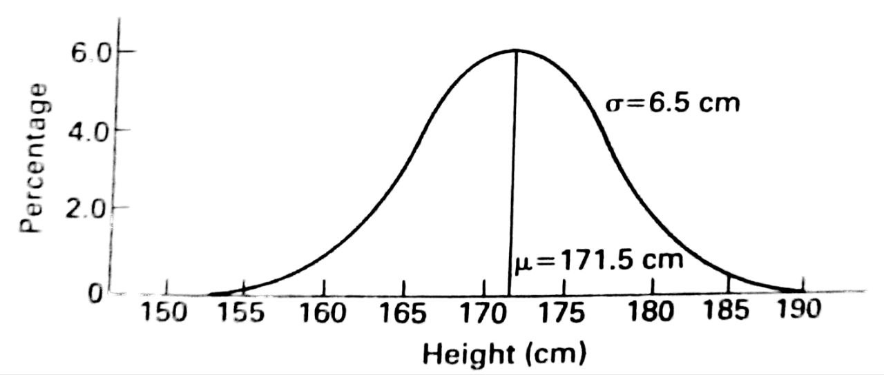
The curve of the normal distribution is symmetrical about the mean and bell-shaped; the bell is tall and narrow for small standard deviations, and short and wide for large ones. Figure 4.1 below illustrates the normal curve describing the distribution of heights of adult men in the United Kingdom.

Other examples of variables that are approximately normally distributed are blood pressure, body temperature, and haemoglobin levels. Examples of variables that are not normally distributed are triceps skinfold thickness and income, both of which are positively skewed.

Sometimes transforming a variable, for example by taking logarithms, will make its distribution more normal. This is described in Chapter 19 “Transformations”, and how to asses whether a variable is normally distributed is discussed in Chapter 18 “Goodness of Fit of Frequency Distributions”.

The normal distribution is important not only because it is a good empirical description of many variables, but because it occupies a central role in the techniques of the statistical analysis. For example. it’s the justification for the calculation of the confidence interval which was mentioned in Chapter 3 and which is described in Chapter 5 “Confidence Interval for a Mean”. It also forms the basis of the methodology of significance testing of means which is introduced in Chapter 6 “Significance Tests for a Single Mean”.

For these reasons it is important to describe the use of the normal distribution in some detail before proceeding further, although the precise mathematical equation which defines it need not be a concern as tables are available.

The Standard Normal Distribution

If a variable is normally distributed then a change of units does not affect this. Thus, for example, whether height is measured in centimeters or inches it is normally distributed. Changing the mean simply moves the curve up or down the axis, while changing the standard deviation alters the height and widths of the curve.

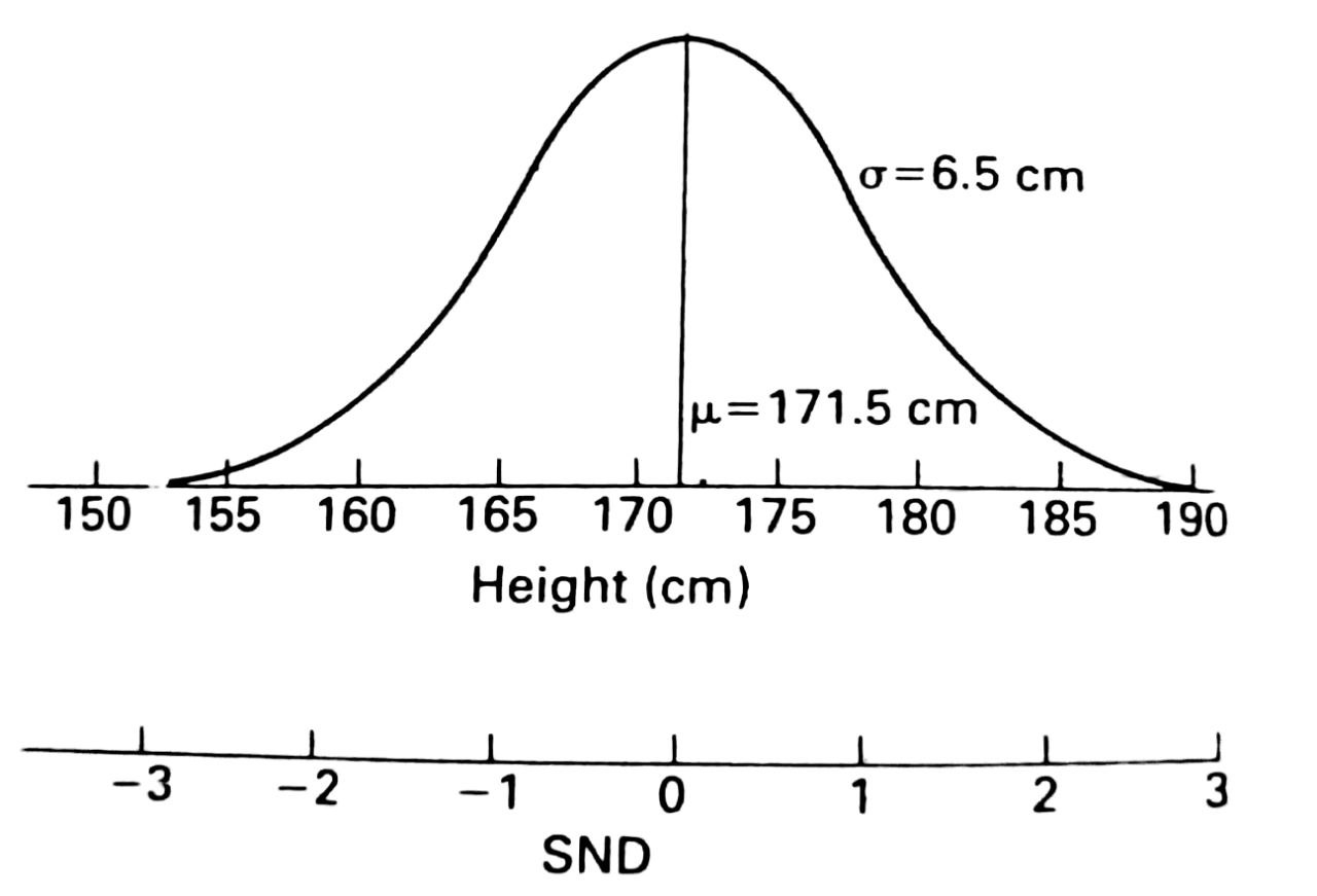
In particular, by a suitable change of units any normally distributed variable can be related to the standard normal distribution whose mean is zero and whose standard deviation is 1. this is done by subtracting the mean from each observation and dividing by the standard deviation.

$$ \textit{SND, z} = \frac{x-\mu}{\sigma} $$

Where $x$ is the original variable with mean $\mu$ and standard deviation $\sigma$ and z is the corresponding standard normal deviate (SND). This is illustrated for the distribution of adult male heights in Figure 4.2 below.

The possibility of converting any normally distributed variable into an SND means that tables are only needed for the standard normal distributions and not for all possible combinations of different values of means and standard deviations.

The two most commonly provided sets of tables are:

• The area under the frequency distribution curve
• The so-called percentage points

Table for Area Under the Curve of the Normal Distribution

The table for the area under the frequency distribution curve of the normal distribution is useful for determining the proportion of the population which has values in specified range. This will be illustrated for the distribution shown in Figures 4.1 and 4.2 of the heights of adult men in the United Kingdom, which is approximately normal with mean $\mu = 171.5$ cm and standard deviation $\sigma = 6.5$ cm.

Area in Upper Tail of Distribution

The normal distribution can be used to estimate, for example, the proportion of men taller than $180$ cm. This proportion is represented by the fraction of the area under the frequency distribution curve that is above $180$ cm.

The corresponding SND is;

$$ \begin{align*} &z = \frac{180-171.5}{6.5} \ &z = 1.31 \ \end{align*} $$

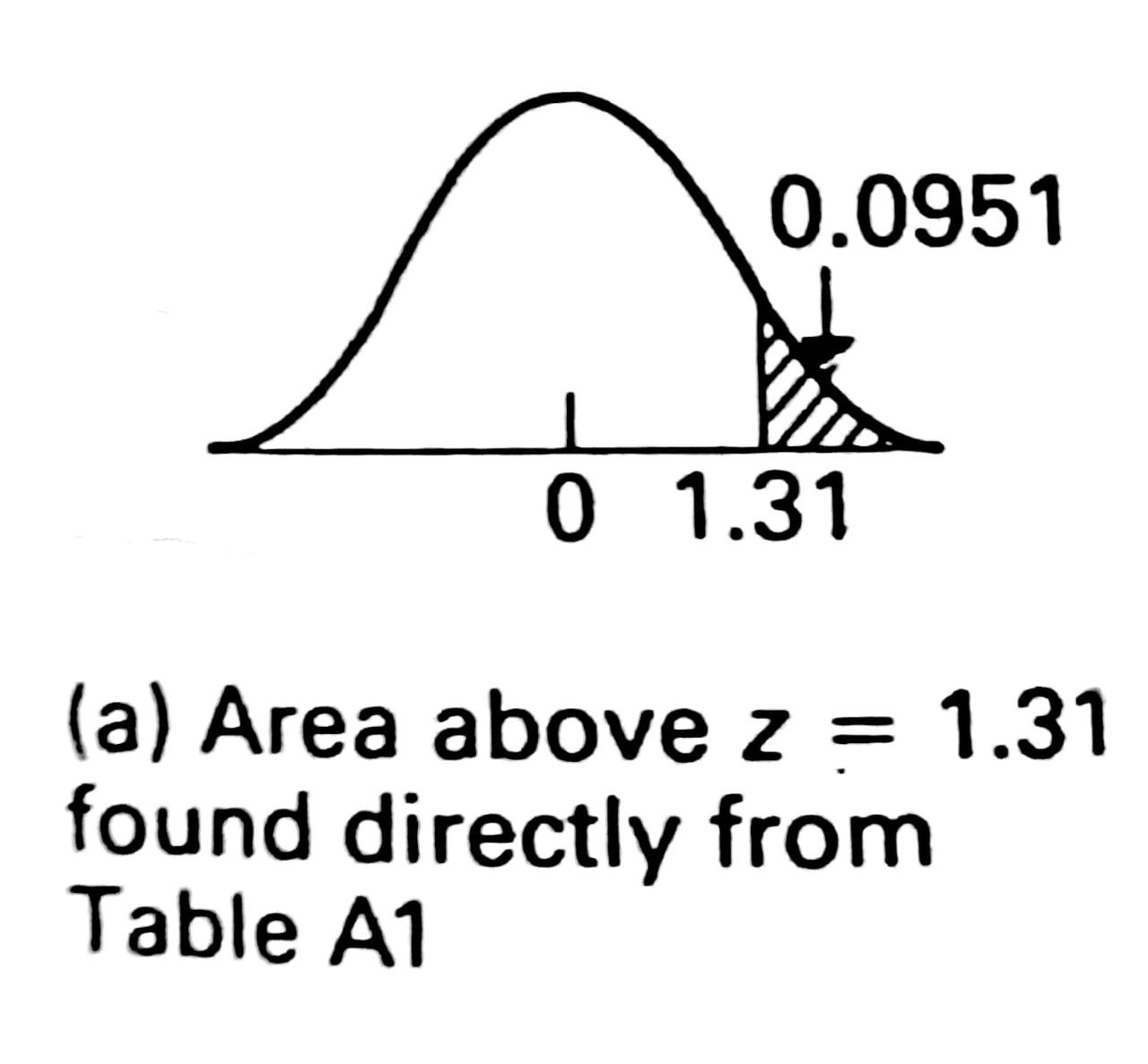
This is equivalent to the proportion of the area of the standard normal distribution that is above $1.31$. This area is illustrated in Figure 4.3 (a) and can be found from Table A1. The rows of the table refers to $z$ to one decimal place and the columns to the second decimal place. Thus the area above $1.31$, given in row 1.3 and column 0.01, is $0.0951$. We conclude that a fraction $0.0951$, or equivalently $9.51%$, of adult men are taller than $180$ cm.

Area in the Lower Tail of Distribution

The proportion of men shorter than $160$ cm, for example can be similarly estimated.

$$ \begin{align*} &z = \frac{160-171.5}{6.5} \ &z = -1.77 \ \end{align*} $$

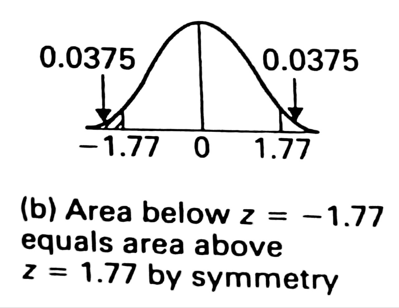
The required area is illustrated in Figure 4.3 (b) above. As the standard normal distribution is symmetrical about zero the area below $z = -1.77$ is equal to the area above $z - 1.77$ which is $0.0375$. Thus $3.75%$ of men are shorter than $160$ cm.

Area of Distribution Between Two Values

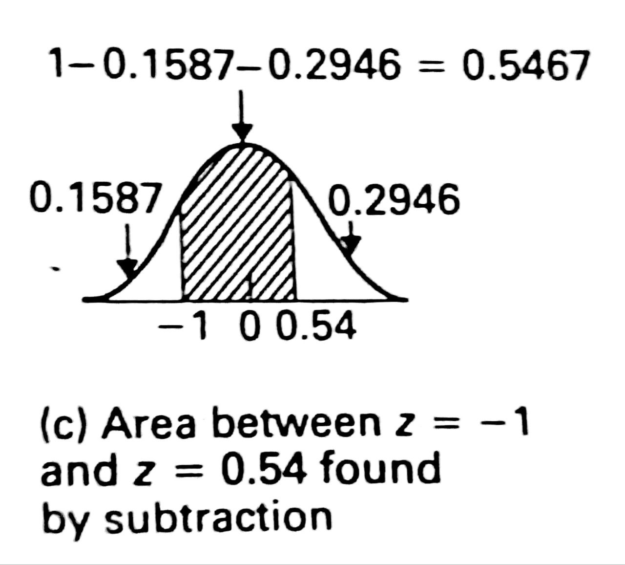
The proportion of men with a height between, for example, $165$ cm and $175$ cm is estimated by finding the proportions of men shorter than $165$ cm and taller than $175$ cm and subtracting these from $1$.

(i) SND corresponding to $165$ cm is:

$$ \begin{align*} &z = \frac{165 - 171.5}{6.5}&& \ &z = -1&& \end{align*} $$

Proportion below this height is $0.1587$.

(ii) SND corresponding to $175$ cm is:

$$ \begin{align*} &z = \frac{175 - 171.5}{6.5}&& \ &z = 0.54&& \end{align*} $$

Proportion above this height is $0.2946$.

(iii) Proportion of men with heights between 165 cm and 175 cm

$$ \begin{align*} &= 1 - \textit{proportion below 165 cm } - \textit{proportion below 175 cm}&& \ &= 1 - 0.1587 - 0.2946&& \ &= 0.5467 \textit{ or } 54.67%&& \end{align*} $$

Value Corresponding to Specified Tail Area

Table A1 can also be used the other way round, that is starting with an area and finding the corresponding $z$ value. For example, what height is exceeded by 5% or 0.05 of the population? Looking through the table the closest value to 0.05 is found 1.6 and column 0.04 and so the required $z$ value is $1.64$.

The corresponding height is found by inverting the definition of SND to give:

$$ x = \mu + z \times \sigma $$

and is $171.5 + 1.64 \times 6.5 = 182.2$ cm.

Percentage points of the Normal Distribution

An interpretation of the SND that is sometimes useful is that it expresses the value of the variable in terms of the number of standard deviations it is away from the mean. This is shown on the scale of the original variable in Figure 4.4 below.

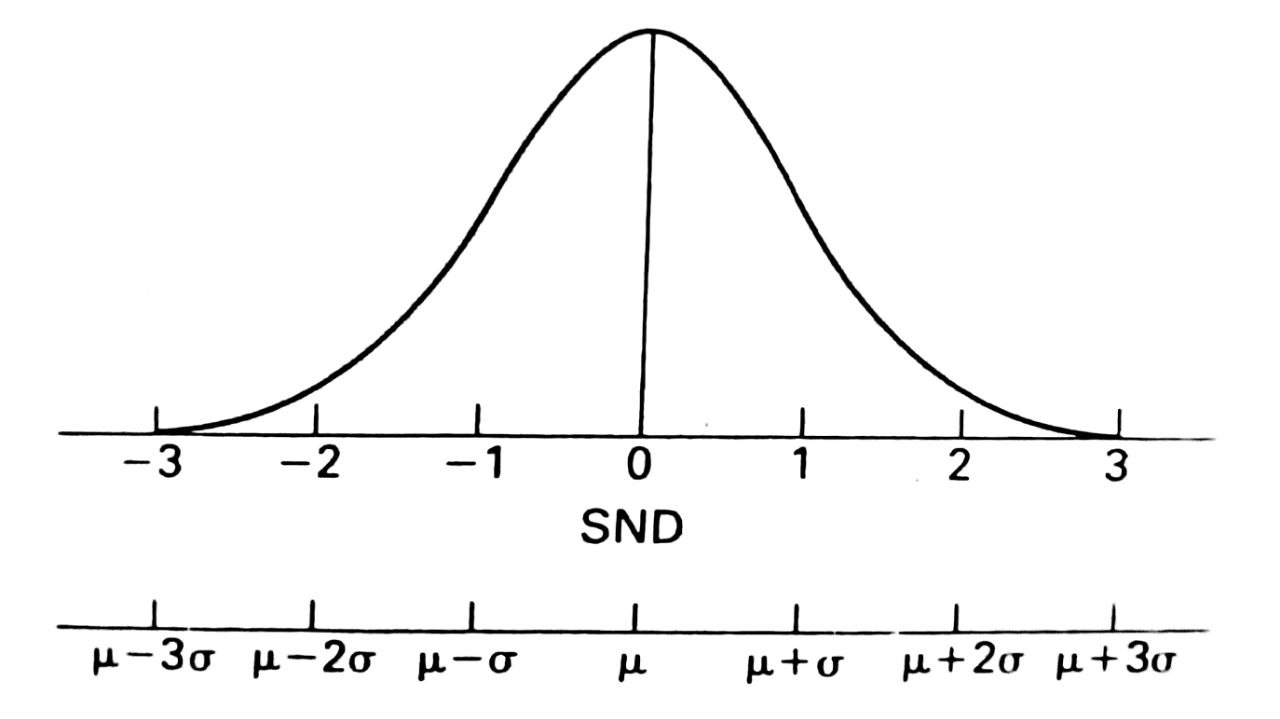
Thus for example, $z = 1$ corresponds toa value which is one standard deviation above the mean and $z = -1$ to one standard deviation below the mean. The areas above $z = 1$ and below $z = -1$ are both $0.1587$ or $15.87%$. Therefore 31.74% ($2 \times 15.87%$) of the distribution is further than one standard deviation from the mean, or equivalently $68.26%$ of the distribution lies within one standard deviation of the mean.

Similarly, $4.55%$ of the distribution is further than two standard deviations from the mean, or equivalently $95.45%$ of the distribution lies within two standard deviations of the mean.

These are the justifications for the practical interpretations of the standard deviation given in Chapter 3.

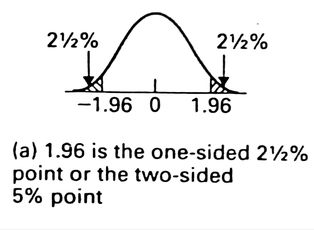
The $z$ value encompassing exactly $95%$ of the distribution between $-z$ and $z$ is 1.96, shown in figure 4.5 (a) below. 1.96 is said to be the 5% percentage point of the normal distribution, as $5%$ of the distribution is further than 1.96 standard deviations from the mean ($2.5%$ in each tail).

Similarly, 2.58 standard deviations away from the mean is the $1%$ percentage point of the normal distribution ($0.5%$ in each tail). The commonly used percentage points are tabulated in Table A2. Note that they could also be found from Table A1 in the way described above.

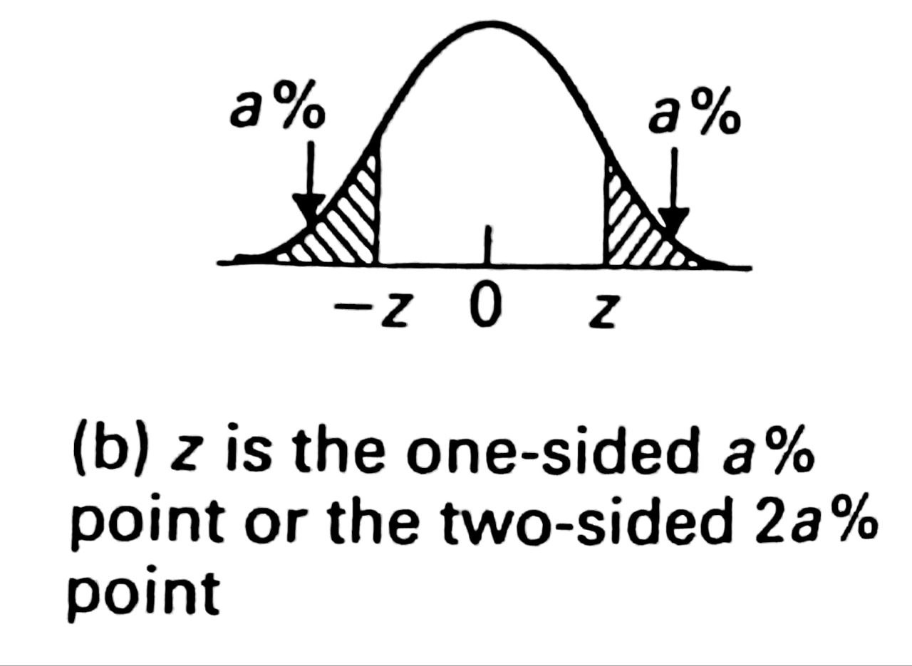
The percentage points described here are known as two-sided percentage points, as they cover extreme observations in both upper and lower tails of the distribution. Some books tabulate one-sided percentage points, referring to just one tail of the distribution.

The one sided a% point is the same as the two-sided 2a% point, illustrated below in figure 4.5 (b).

For example, 1.96 is the one-sided 2.5% point, as 2.5% of the standard normal distribution is above 1.96 (or equivalently 2.5% is below -1.96) and it is the two-sided 5% point. This difference is discussed again in Chapter 6 “Significance Tests for a Single Mean” in the context of significance testing.