Introduction

A frequency distribution gives a general picture of the values of a variable. It is often convenient, however, to summarize a quantitave variable still further by giving just two measurements, one indicating the average value and the other the spread of the values.

Mean, Median, and Mode

The average value is usually represented by the arithmetic mean, customarily just called the mean. This is simply the sum of the values divided by the number of values.

$$ Mean, \bar{x} = \frac{\Sigma x}{n} $$

Where x denotes the values of the variable, Sigma (the Greek capital letter sigma) means ’the sum of’ and n is the number of observations. The mean is denoted by $\bar{x}$ (spoken ‘x bar’).

Other measures of the average value are the median and the mode. The median is the value that divides the distribution in half. If the observations are arranged in increasing order, the median is the middle observation.

$$ Median = \frac{n+1}{2}th\text{ value of ordered observations} $$

If there is an even number of observations, there is no middle one and the average of the two ‘middle’ ones is taken. The mode is the value which occurs most often.

[!example]+ Example 3.1 The following are the plasma volumes in liters of eight healthy adult males: $$\text{2.75, 2.86, 3.37, 2.76, 2.62, 3.49, 3.05, 3.12}$$

(a) Getting the mean

$$ \begin{align*} &\text{n = 8}&& \\ &\Sigma x = 2.75 + 2.86 + 3.37 + 2.76 + 2.62 + 3.49 + 3.05 + 3.12&& \\ &\Sigma x = 24.02&& \\ &Mean, \bar{x} = \frac{\Sigma x}{n} = \frac{24.02}{8} = 3.00 \text{ liters}&& \end{align*} $$

(b) Getting the median

$$ \begin{align*} &\textbf{Rearranging the measurements in increasing order gives:}&& \\ &\text{2.62, 2.75, 2.76, 2.86, 3.05, 3.12, 3.37, 3.49}&& \\ \end{align*} $$

$$ \begin{align*} &Median = \frac{n + 1}{2} = \frac{9}{2} = \textit{ 4.5th value}&& \\ &Median = \textit{average of the 4th and 5th values}&& \\ &Median = \frac{(2.86 + 3.05)}{2} = 2.961&& \end{align*} $$

(c) There is no estimate of the mode, since all the values are different.

The mean is usually preferred measure since it takes into account each individual observation and is most amenable to mathematical and statistical techniques.

The median is a useful descriptive measure if there are one or two extremely high or low values, which would make the mean unrepresentative of the majority of the data.

The mode is seldom used. If the sample is small, either it may not be possible to estimate the mode (as in the example above), or the estimate obtained may be misleading.

The mean, median, and mode are, on average, equal, however, when the distribution is symmetrical and unimodal. When the distribution is positively skewed, a geometric mean is more appropriate than the arithmetic mean. This is discussed in Chapter 19 “Transformations”.

Measure of Variation

The simplest measure of variation is the range, which is the difference between the largest and smallest values. Its disadvantages is that it is based on only two of the observations and gives no idea of how the other observations are arranged between these two. Also, it tends to be larges, the larger the size of the sample.

Since the variation is small if the observations are bunched closely about their mean, and large if they are scattered over considerable distances, variation is measured instead in terms of the deviations of the observations from the mean. The variance is the average of the squares of these differences.

When calculating the variance of a sample, the sum of squared deviations is divided by $(n-1)$ rather than $n$, however, because this gives a better estimate of the variance of the total population.

$$ Variance, s^2 = \frac{\Sigma (x-\bar{x})^2}{(n-1)} $$

Degrees of Freedom

The denominator $(n-1)$ is called the number of degrees of freedom of the variance. This number is $(n-1)$ rather than $n$, since only $(n-1)$ of the deviations $(x-\bar{x})$ are independent from each other. The last one can always be calculated from the others because all $n$ of them must add up to zero.

Standard Deviation

The variance has convenient mathematical properties and is the appropriate measure when doing statistical theory. A disadvantage, however, is that it is in the square of the units used for the observations. If the observations are weights in grams, the variance is in grams squared. For many purposes it is more convenient to express the variation in the original units by taking the square root of the variance. This is called the standard deviation (s.d.)

$$ \textit{s.d., s} = \sqrt{\left[\frac{\Sigma (x - \bar{x})^2}{(n-1)}\right]} \\\ \\\ \textbf{or equivalently} \\\ \\\ \textit{s.d., s} = \sqrt{\left[\frac{\Sigma x^2 - \frac{(\Sigma x)^2}{n}}{(n-1)}\right]} $$

The latter is a more convenient form for calculation, since the mean does not have to be calculated first and then subtracted from each of the observations.

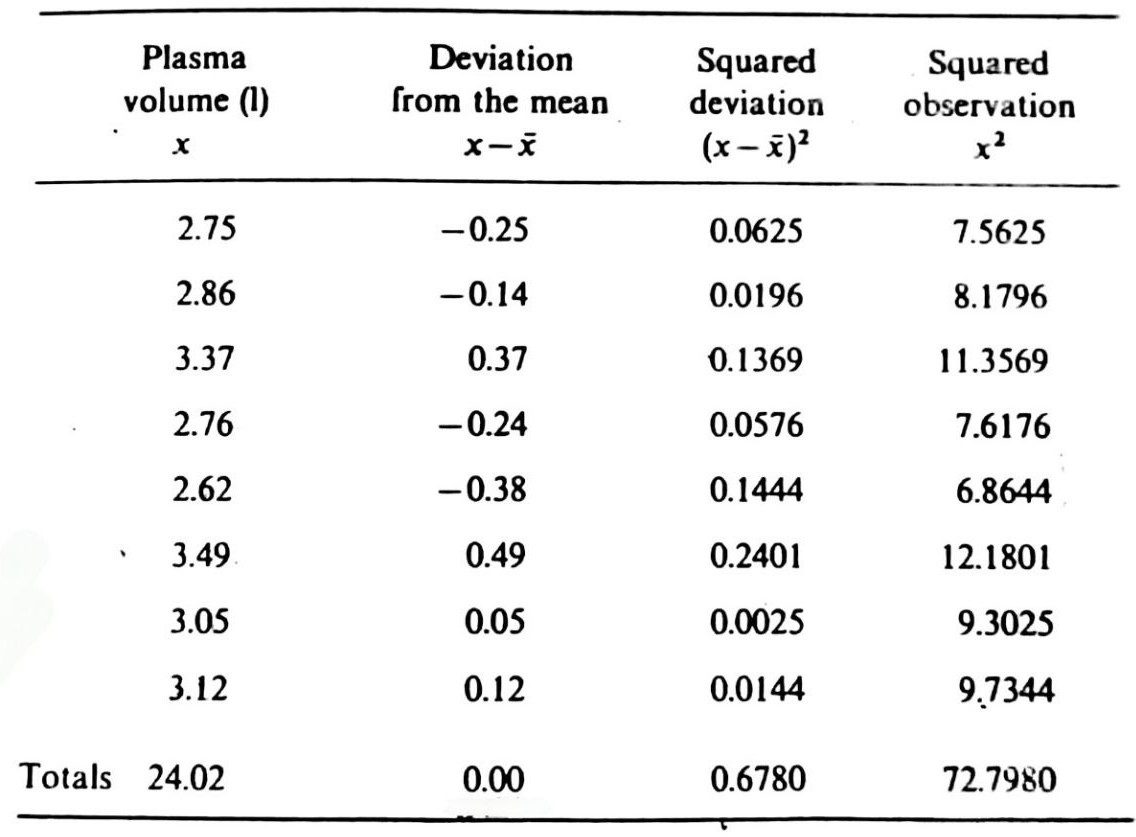
[!example]+ Example 3.2 Table 3.1 below shows the steps for the calculation of the standard deviation of the eight plasma volume measurements of Example 3.1

$$ \begin{align*} &\textit{s.d.} = \sqrt{\left[\frac{\Sigma x^2 - \frac{(\Sigma x)^2}{n}}{(n-1)}\right]}&& \\ &\textit{s.d.} = \sqrt{\left[\frac{72.7980 - \frac{(24.02)^2}{8}}{(8-1)}\right]}&& \\ &\textit{s.d.} = \sqrt{\left[\frac{0.6780}{7}\right]}&& \\ &\textit{s.d.} = \sqrt{0.096857}&& \\ &\textit{s.d.} = 0.31&& \\ \end{align*} $$

^6793fa

Interpretation

Usually about 70% of the observations lie within one standard deviation of their mean, and about 95% lie within two standard deviants. These figures are based on a theoretical frequency distribution, called the normal distribution, which is described in {<{ link “Chapter 4” “the normal distribution” >}}.

Coefficient of variation

$$ c.v = \frac{s}{\bar{x}}\times100 $$ The coefficient variation expresses the standard deviation as a percentage of the sample mean. This is useful when interest is in the size of the variation relative to the size of the observation, and it has the advantage that the coefficient of variation is independent of the units of observation.

[!example]+ Example 3.3 The value of the standard deviation of a set of weights will be different depending on whether they are measured in kilograms or pounds. The coefficient of variation, however, will be the same in the two units.

Calculating the Mean and Standard Deviation from a Frequency distribution

Table 3.2 below shows the distribution of the number of previous pregnancies of a group of women attending an antenatal clinic. Eighteen of the 100 women had no previous pregnancies, 27 had one, 31 had two, 19 had three, and 5 had four previous pregnancies.

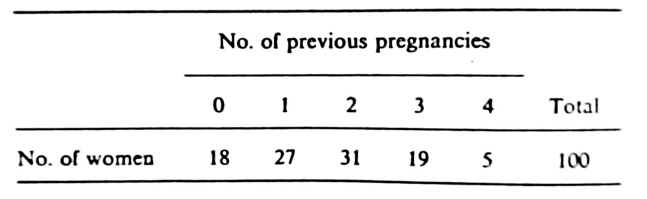As, for example, adding 2 thirty-one times is equivalent to adding the product ($2 \times 31$), therefore the total number of previous pregnancies is calculated by:

$$ \begin{align*} &\Sigma x = (0\times18) + (1\times27) + (2\times31) + (3\times19) + (4\times5)&& \\ &\Sigma x = 0 + 27 + 62 + 57 + 20&& \\ &\Sigma x = 166&& \end{align*} $$

The mean of previous pregnancies is then:

$$ \begin{align*} &\bar{x} = 166/100&& \\ &\bar{x} = 1.66 \end{align*} $$

In the same way the standard deviation can be calculated:

$$ \begin{align*} &\textbf{Formula}&& \\ &\textit{s.d., s} = \sqrt{\left[\frac{\Sigma x^2 - \frac{(\Sigma x)^2}{n}}{(n-1)}\right]} \\ \\ \hline&& \\ &\textbf{Steps}&& \\ &\Sigma x^2 = (0^2\times18) + (^2\times27) + (2^2\times31) + (3^2\times19) + (4^2\times5)&& \\ &\Sigma x^2 = 0 + 27 + 124 + 171 + 80&& \\ &\Sigma x^2 = 402 \\ &\textbf{————}&& \\ &\textit{s.d., s} = \sqrt{\left[\frac{402 - \frac{166^2}{100}}{(100-1)}\right]}&& \\ &\textit{s.d., s} = \sqrt{\left[\frac{126.44}{99}\right]}&& \\ &\textit{s.d., s} = 1.13&& \end{align*} $$

If the variable has been grouped when constructing a frequency distribution, its mean and standard deviation should be calculated using the original values, not the frequency distribution. There are occasions, however, when only the frequency distribution is available. In such a case, approximate values for the mean and standard deviation can be calculated by using the values of the mid-points of the groups and proceeding as above.

Change of Units

Adding or subtracting a constant from the observations alters the mean by the same amount but leaves the standard deviation unaffected. Multiplying or dividing by a constant changes both the mean and the standard deviation in the same way.

[!example]+ Example 3.4 Suppose a set of temperatures is converted from Fahrenheit to centigrade. This is done by subtracting 32, multiplying by 5, and dividing by 9.

The new mean may be calculated from the old one in exactly the same way, that is by subtracting 32, multiplying by 5, and dividing by 9.

The new standard deviation, However, is simply the one multiplied by 5 and divided by 9, since the subtraction does not affect it.

Sampling Variation and Standard Error

As discussed in Chapter 1, the sample is of interest not in its own right, but for what it tells the investigator about the population which it represents. The sample mean ($\bar{x}$), and standard deviation ($s$) are used to estimate the mean and standard deviation of the population, denoted by the Greek letters $\mu$ (mu) and $\sigma$ (sigma) respectively.

The sample mean is unlikely to be exactly equal to the population mean. A different sample would give a different estimate, the difference being due to sampling variation. Imagine collecting many independent samples of the same size and calculating the sample mean of each of them. A frequency distribution of these means could then be formed. The mean of of this distributions would be the population mean, and it can be shown that its standard deviation would equal $\frac{\sigma}{\sqrt{n}}$. This is called the standard error of the sample mean, and it measures how precisely the population mean is estimated by the sample mean.

The size of the standard error depends both on how much variation there is in the population and on the size of the sample. The larger the sample, the smaller is the standard error.

We seldom know the population standard deviation ($\sigma$), however, and so we use the sample standard deviation ($s$) to estimate the standard error.

$$ s.e. = \frac{s}{\sqrt{n}} $$

[!example]+ Example 3.5 The mean of the eight plasma volumes shown in Table 3.1 is 3.00 and the standard deviation is 0.31. The standard error of the mean is therefore estimated as:

$$ \begin{align*} &s.e = \frac{0.31}{\sqrt{8}}&& \\ &s.e = 0.11&& \end{align*} $$

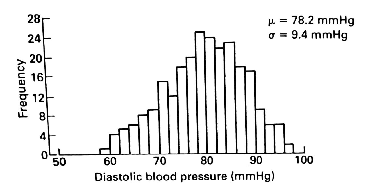
[!example]+ Example 3.6 A game played with a class of 30 students to illustrate the concepts of sampling variants, the sampling distribution, and the standard error. Blood pressure measurements for 250 airline pilots were used.

The distribution of these measurements is show in Figure 3.1 (a) below. The population mean ($\mu$) was 78.2 mmHg, and the population standard deviation ($\sigma$) was 9.4 mmHg. Each value was written on a small disc and the 250 discs put into a bag.

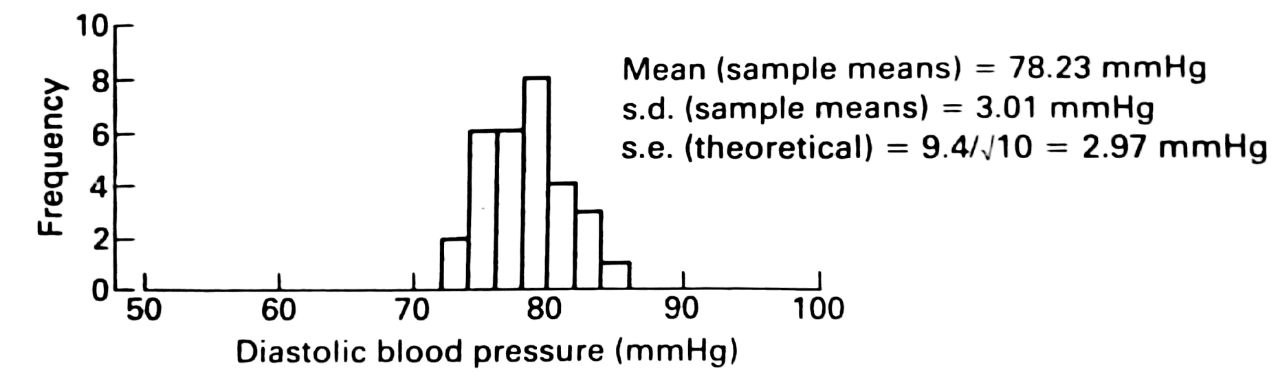
Each student was asked to shake the bag, select 10 discs, write down the 10 diastolic pressures, work out their mean ($\bar{x}$), and return the discs to the bag. In this way 30 different samples were obtained, with 30 different sample means, each estimating the same population mean. The means of these samples means was 78.23 mmHg , close to the population mean. Their distribution is show in Figure 3.1 (b) below.

The standard deviation of the sample means was 3.01 mmHg, which agreed well with the theoretical value, $\frac{\sigma}{\sqrt{n}} = \frac{9.4}{\sqrt{10}} = 2.97 \text{ mmHg}$, for the standard error of the mean of a sample of size 10.

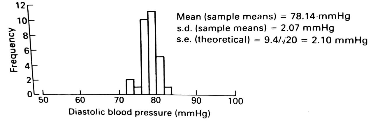
The exercise was repeated taking samples of size 20. The results are show in Figure 3.1 (c) below.

The reduced variation in the sample means resulting from increasing the sample size from 10 to 20 can be clearly seen. The mean of he sample means was 78.14 mmHg, again close to the population mean. The standard deviation was 2.07 mmHg, again in good agreement with the theoretical value, $\frac{9.4}{\sqrt{20}} = 2.10 \text{ mmHg}$.

Interpretation

The interpretation of the standard error of a sample mean is similar to that of the standard deviation. Approximately 95% of the sample means obtained by repeated sampling would lie within two standard errors above or below the population mean.

Finite Population Correction

If a sample is from a population of finite size, for example the houses in a village, the sampling variation is considerably smaller than $\frac{\sigma}{\sqrt{n}}$ when a large proportion of the population is sampled. It would be zero if the whole population were sampled, not because there is not variation among individuals in the population, but because the sample meanis then the population mean.

A second sample of the same size (i.e. the whole population) would automatically give the same result. A finite population correction (f.p.c.) is therefore applied when working out the standard error. The formula becomes:

$$ \textit{s.e with f.p.c.} = \frac{\sigma}{\sqrt{n}} \times \sqrt{\left(1-\frac{n}{N}\right)} $$ $$ \text{where N is the population size and } \frac{n}{N} \text{ is the sampling fraction} $$

Ignoring the finite population correction results in an overestimation of the standard error.

[!example]+ Example 3.7 If 75% of the population were sampled, the finite population correction would equal $\sqrt{(1-0.75)} = 0.5$. If this were omitted, the standard error estimated would be twice the correct value.

However, the correction has little effect and can be ignored when the sampling fraction is smaller than about 10%.

Summary

• Standard Deviation quantifies the variation within a set of measurements.
• Standard Error quantifies the variation in the means from multiple sets of measurements.
• Confidence Interval is a range of estimates for unknown parameter. In this case it’s the population mean ($\mu$).

Useful Resources

• Understanding standard errors